PBR for Audio Software Interfaces

This article describes our rendering system. Reading time = 5 min.

The User Interface (UI) of the last Auburn Sounds audio plug-ins are fully rendered. This rendering is heavily inspired by Physically Based Rendering (PBR), used in today's video games.

This whole system can be bypassed, in which case the rendering become similar to IPlug instead.

1. Why PBR?

Quite unsurprisingly, audio plug-ins are primarily about audio processing.

Yet all things being equal, it is still valuable to have a good-looking user interface. More press coverage, users liking the sound more, users sharing more on social networks: the benefits are seemingly endless.

What PBR does is taking average graphics as input, giving back more aesthetically pleasing images in a systematic way.

2. Other approaches

Audio plug-ins UI are expected to be — much like video games — pretty, unique and identical across platforms. How is it usually done?

Alternative Option 1: Pre-rendering widget states

A common way to render widgets in plug-ins UI is to use pre-rendered widgets in every possible state. For example this was a potentiometer knob texture used for one of our former plug-ins:

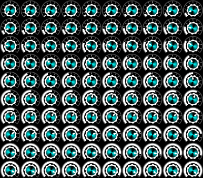
Here the widget graphics need to be stored in memory and disk 100 times. For this very reason, plug-in installations are often found over 100MB in size.

The primary goal of using PBR was to reduce installation size. With PBR, widgets can use an order-of-magnitude less memory and disk space, because only the current state gets rendered.

While users rarely complain about large binaries, beta-testing, hosting and downloading all get easier with small file sizes.

Alternative Option 2: OpenGL

An alternative to pre-rendering widget states is to redraw everything with an accelerated graphics API like OpenGL. This technology enables the largest real-time updates on screen and potentially the nicest graphics.

However, OpenGL exposes developers to graphics drivers bugs. The “bug surface” of applications becomes a lot larger, while some users are inevitably left behind because of inadequate drivers.

3. Input channels

In order to begin compositing, our renderer requires 9 channel inputs to be filled with pixel data:

• Depth
• Base Color (red, green and blue)
• Physical
• Roughness
• Metalness
• Specular
• Emissive

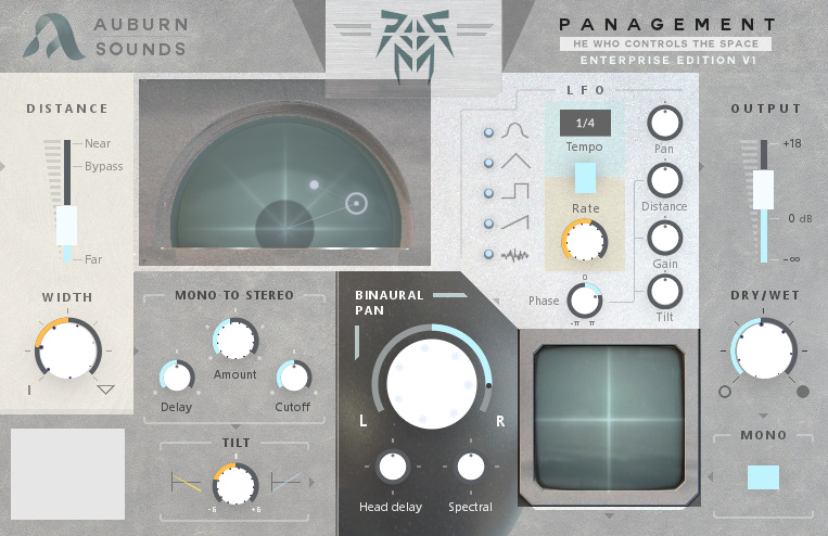
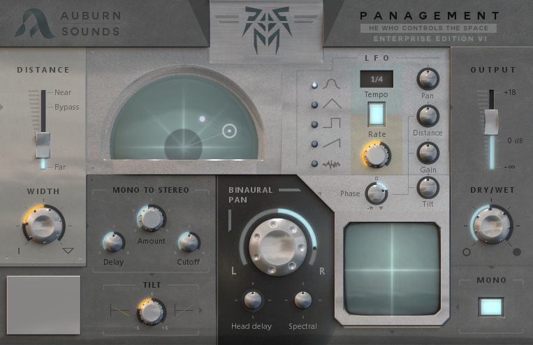
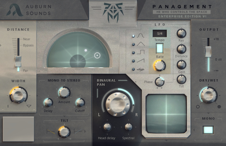
Panagement will be used throughout the rest of the article as an example.

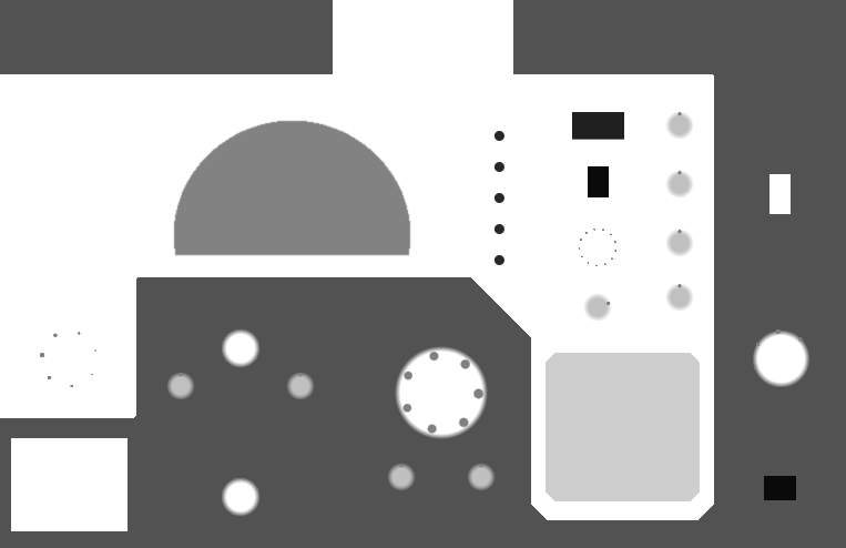
Depth

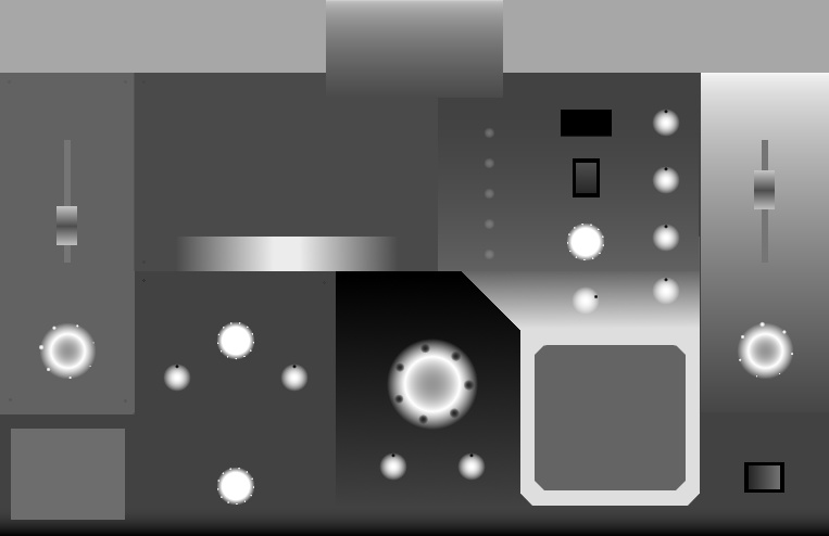
The Depth channel describes the elevation: the whiter, the higher. Originally Depth was stored in an 8-bit buffer but this was the cause of quantization issues with normals. It is now stored in a 16-bit buffer.

Editing Depth is akin to adding or removing matter.

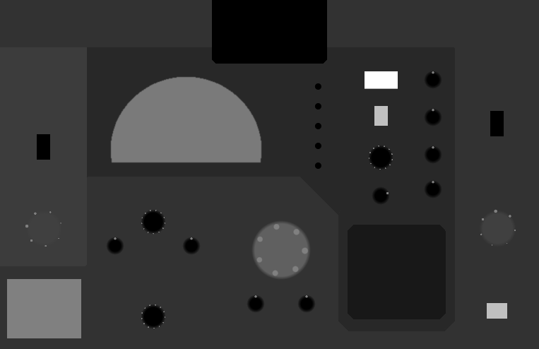
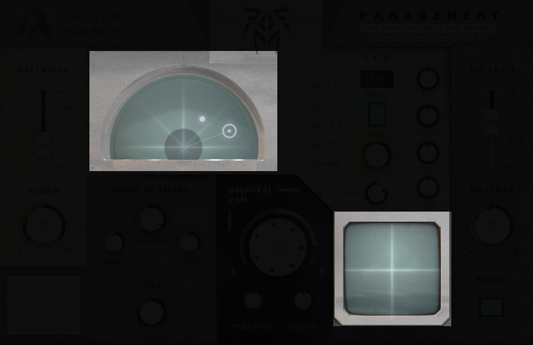
Base Color

Arguably this input requires the most work. The Base Color of the material is also known as “albedo”. This is the appropriate channel for painting labels and markers.

The two darker rectangles are the pre-computed areas. They are manual copies of the same interface parts at a later stage of rendering, fed back into the inputs to gain speed.

Editing Base Color is akin to adding paint.

Physical

The Physical channel signals those pre-computed areas. While rendering, they are copied into the final color buffer with no lighting computation. This saves a lot of processing in the case of continuously updated widgets, where 60 FPS is desirable.

Roughness

The Roughness channel separates rough and soft materials: the whiter, the softer.

Increasing Roughness from left to right.

Metalness

The Metalness channel separates metallic from dielectric materials. The whiter, the more metal. 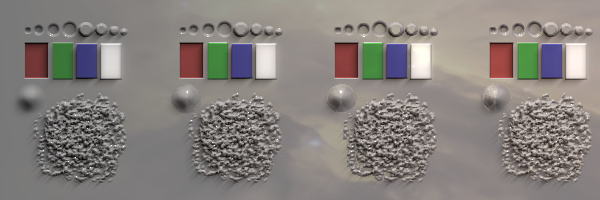Increasing Metalness from left to right.

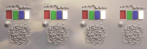
Specular

The Specular channel tells whether the material is shiny. The whiter, the shinier.

You may notice that there is no black in this channel. Rendering practitioners have noticed that Everything is Shiny.

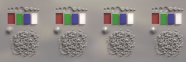Increasing Specular from left to right.

Emissive

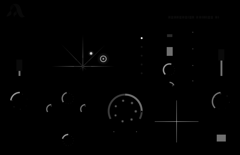The Emissive channel identifies the areas that are emitting light by themselves. As a simplification, the emitted light takes the Base Color as its own color.

Skybox

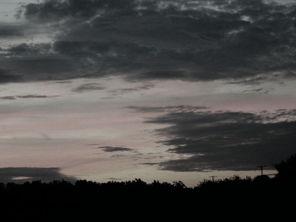A skybox is used to fake environment reflections. It isn't mandatory to take an actual sky picture for this purpose, but this is the case in our example.

All the aforementioned 9 channels are mipmapped for fast access during lighting computations, and organized in a set of 3 different textures (which is helpful for interpolation and look-ups).

4. Lighting computations in our PBR renderer

We'll now describe the 8 steps in which the final color is computed, for each pixel.

Step 1: Getting normals from Depth

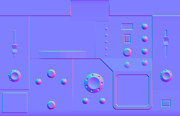
First a buffer of normals is computed using a filtered version of Depth.

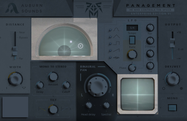
Step 2: Ambient component

Light contributions start with a weak, almost black ambient component.

Note that the pre-computed areas do not partake in this summing, being already shaded.

Step 3: First light

A hard light is cast to make a short-scale shadows appear across the entire UI.

Step 4: Second light

Then another light is cast which is more of a diffuse one.

Step 5: Adding specular highlights

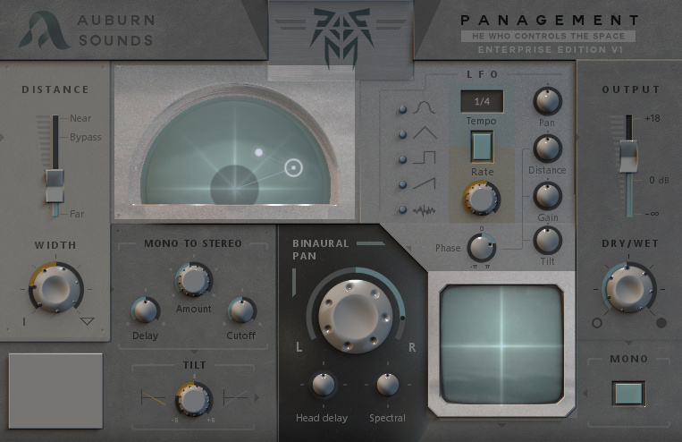
At this moment, specular highlights are added from a third virtual light source, which is only specular.

Step 6: Adding skybox reflections

Skybox reflections gets added, which differentiate the metallic materials from others.

Step 7: Adding light emitted by neighbours

With mipmapping we can add light contributions of neighbouring pixels efficiently. At this stage we can take pixels and put them in another pre-computed area back into the inputs.

The balance is still unsatisfactory because the available color gamut isn't completely used. We need one last step of color correction.

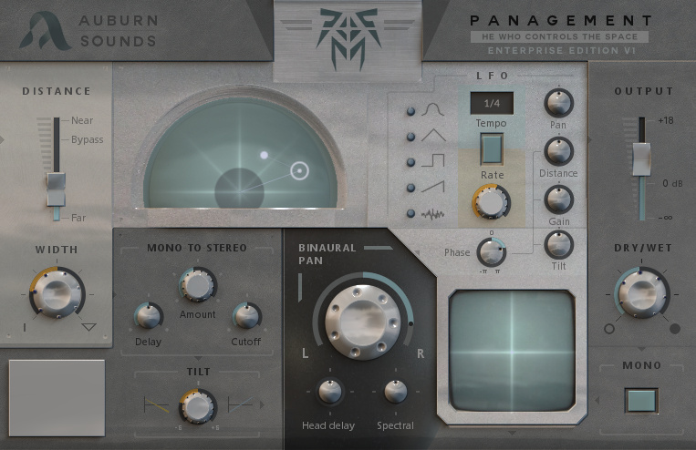
Step 8: Correcting colors

Colors are finally corrected with interactively selected Lift-Gamma-Gain-Contrast curves. This step feels a bit like Audio Mastering in that checking with different users and trying on different screens is helpful.

This is the final output users see.

How fast is this?

This renderer has been optimized thoroughly. Widgets drawing, mipmapping and compositing were all made parallel to leverage multiple cores.

The first opening of Panagement takes about 160 ms and subsequent updates are under 16 ms. When a widget is touched, only an area around it is composited again.

5. Conclusion

PBR comes with natural perks like small file sizes and global lighting control.

It is also complex with a lot of parameters to tune. While the UI becomes flexible, the process of creating it gets more work-intensive.

This renderer is available in the Dplug audio plug-in framework.